A DataSherpas Quick Tip.
In this quick tip article we show you how to hide and unhide columns in Google Sheets. Hiding and unhiding columns is a very simple and quick process and there are even keyboard shortcuts to help speed things up even more.
Let’s get started.
Hiding Columns
Open up your Google Sheet.
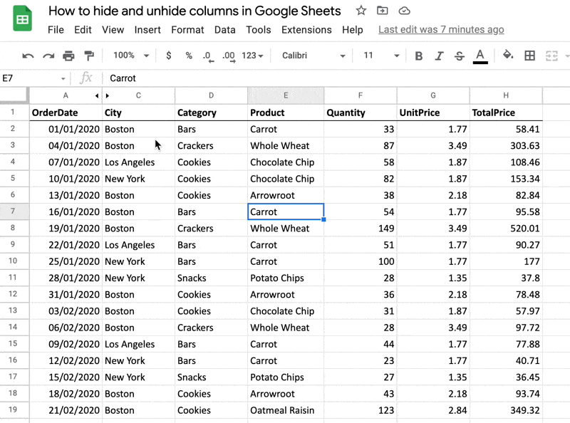
In our example Google Sheet we want to hide column B (Region).
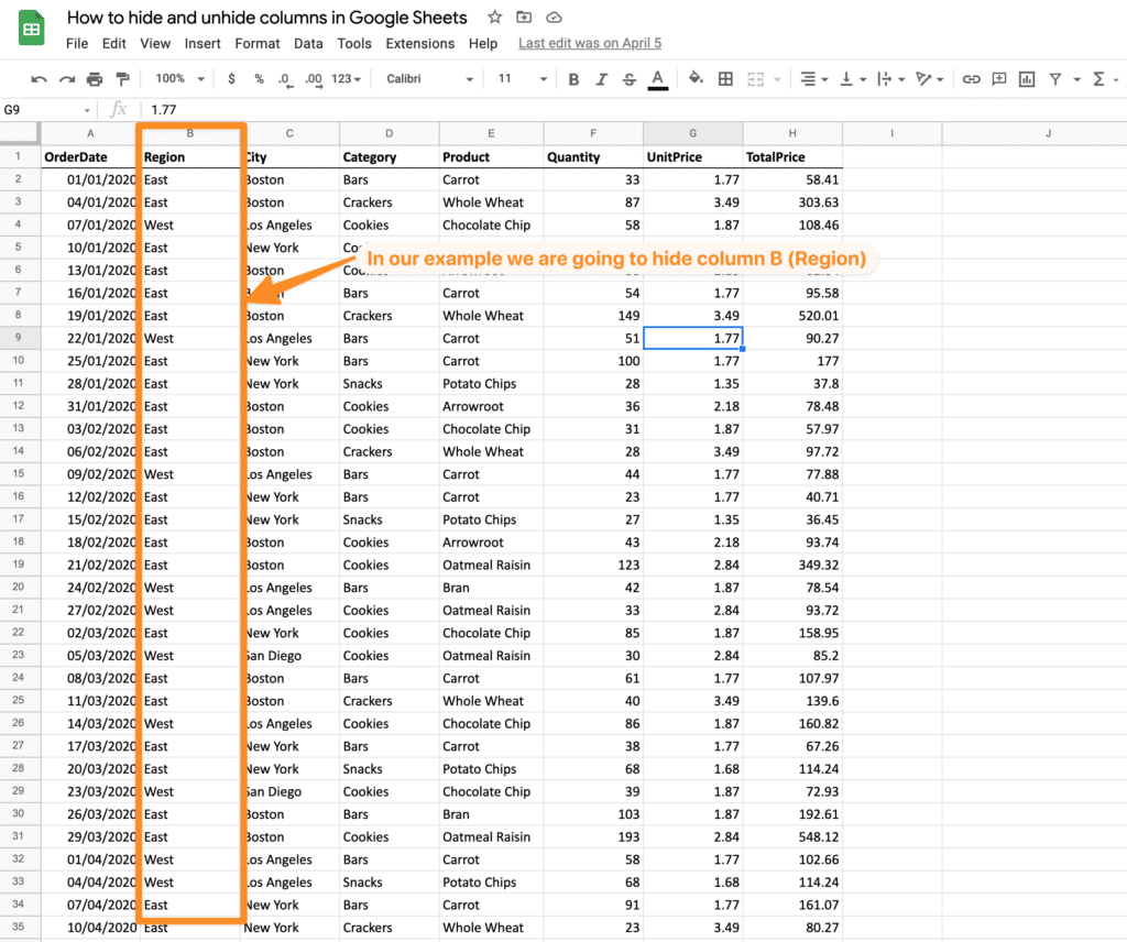
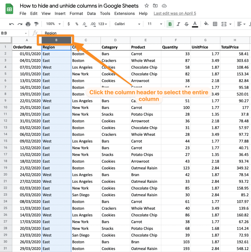
First you will need to select the column. To do that click on the column header (in our example “B”) to select the entire column.
Now with your right mouse button click in the column header again to reveal the options menu. Now choose “Hide Column”.
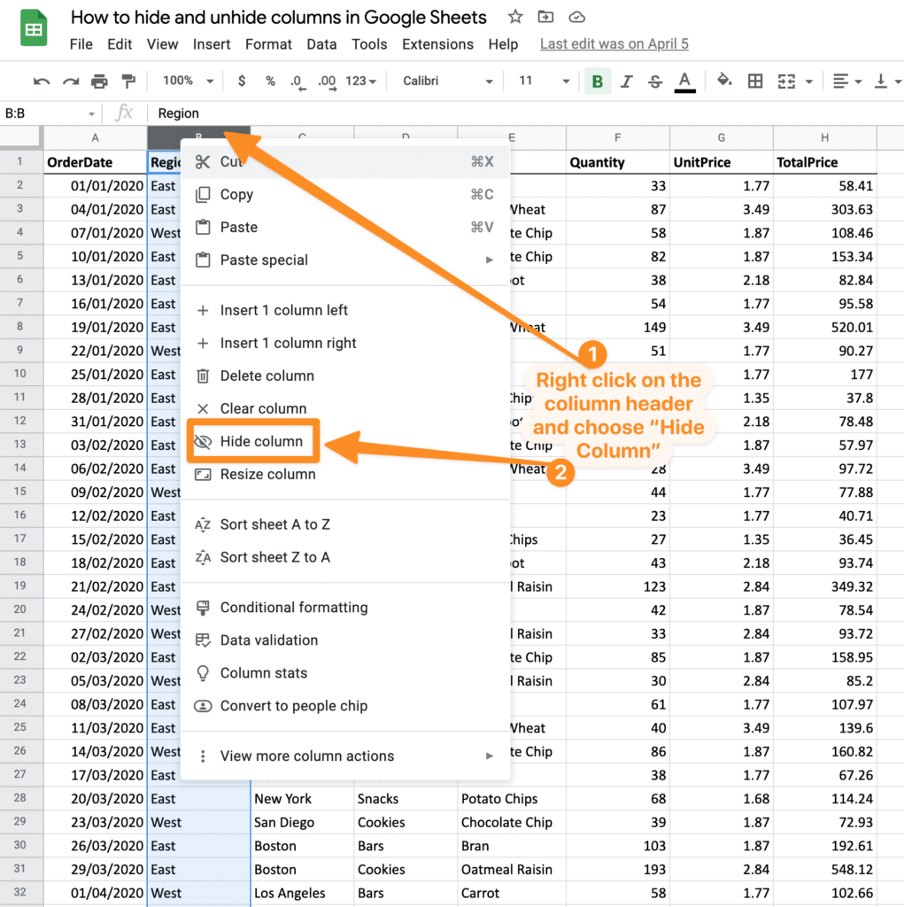
Your selected column will now be hidden.
If you are keyboard shortcut lover you can also do the same using your keyboard.
First select the columns as we did above, by clicking on the column header (in our example we are clicking on the B). Now on your keyboard press the following keys on your keyboard:
Windows / PC: CTRL + ALT + 0 (hold down the CTRL and ALT keys and then press 0)
Mac: CMD + Option + 0 (hold down the COMMAND and Option keys and then press 0)
Your column should be hidden.
Unhiding columns.
Unhiding columns is just as simple as hiding them. Sticking with the same example our column B is currently hidden.
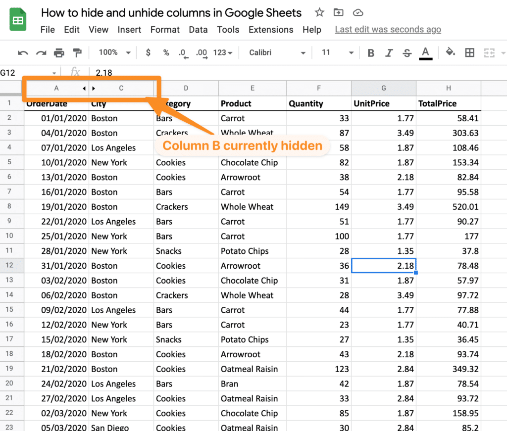
On the column headers where the column that is currently hidden should be, you will see two arrows – one pointing left and the other pointing right. These arrows indicate there is a hidden column and clicking on either one of the arrows will unhide the column.
![]()
You can also unhide columns by selecting the columns to the left and right of the hidden column, pressing your right mouse button and choose “Unhide Columns” from the sub menu.
How to hide all unused columns in Google Sheets
You may have a case where you need to delete all of the unused columns in your Google Sheet.
Let’s use our example Google Sheet again. Now we would like to delete all columns to the right of column H. This will tidy our Google Sheet up a little and enhance the presentation of our data.
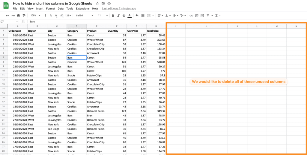
First select the column after (to the right) of the last column that contains the data you want to keep. In our example we select column “I”.
With this column selected now hold down the CTRL + SHIFT (Mac: CMD + SHIFT) Keys and press the right arrow key on your keyboard. This will select all of the unused columns to the right of your selected column.
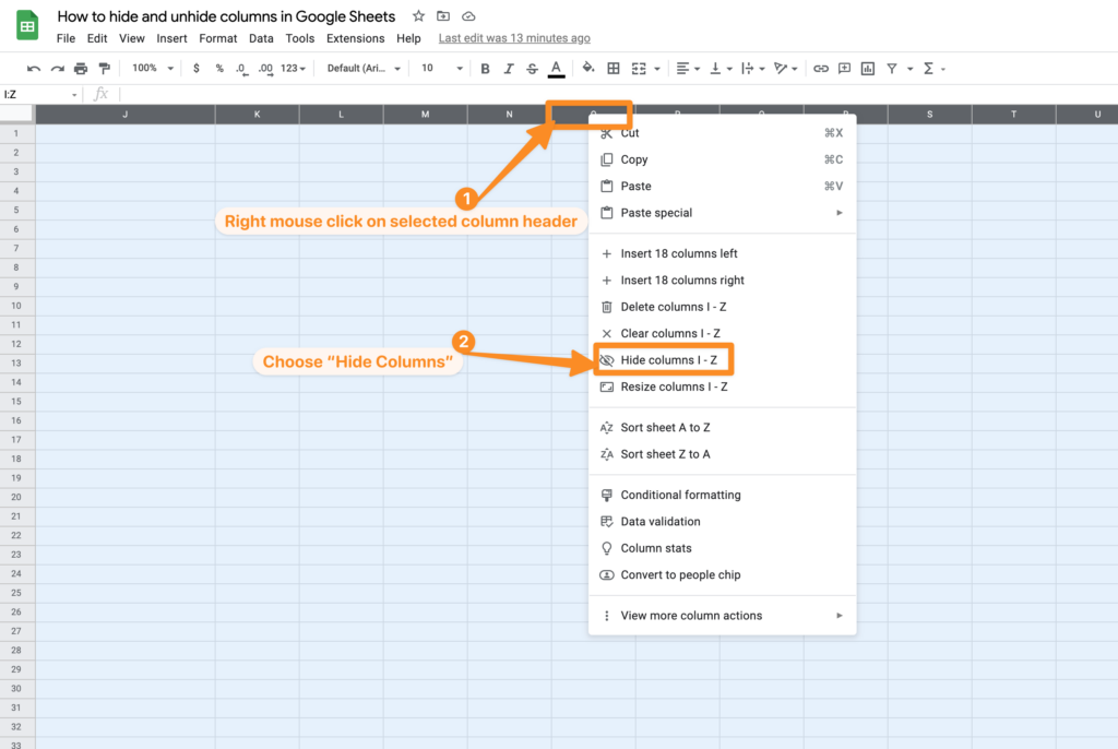
Next right mouse click on any of the column headers of the selected columns and choose “Hide Columns” in our example the choice is “Hide Columns I to Z” – which are the columns that are empty.
(If you are sure the columns are no longer needed you could also delete them instead of hiding).
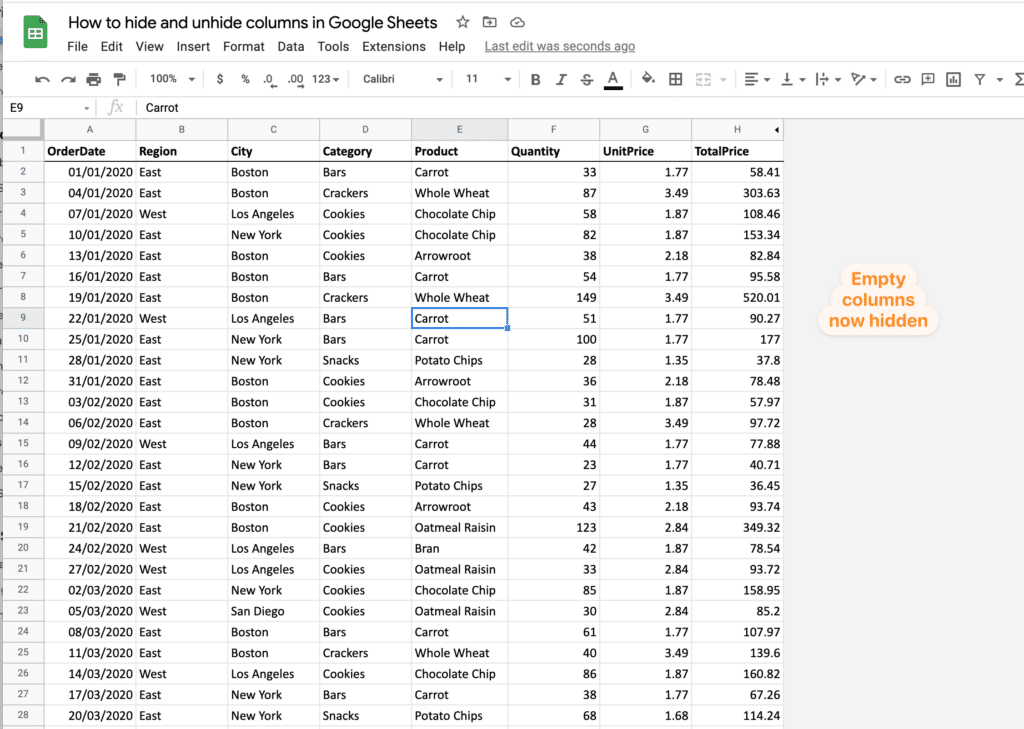
The selected columns will now be hidden.
Other resources
- Official Google support page on hiding columns.
- Our YouTube video with a walk through of hiding and unhiding columns in Google Sheets.
Related Quick Tips
- How to add columns in Google Sheets
- How to freeze columns in Google Sheets
- How to merge cells in Google Sheets.
- How to lock cells in Google Sheets
Hiding columns can be useful in numerous circumstances. It could be to tidy up your Google Sheet and remove unwanted columns. It could be to temporarily hide columns while you work on other columns so there is less noise. Or it could be to make your data more presentable and show just the important data to your Google Sheet users. Whatever your use case we hope this quick tip articles proves useful. If you have any questions or need further help please leave a comment below or contact us via our contact page.