A DataSherpas Quick Tip.
In this quick tip article we explain how to freeze columns in Google Sheets. The process is very similar to that explained in our recent quick tip article – How to freeze a row in Google Sheets.
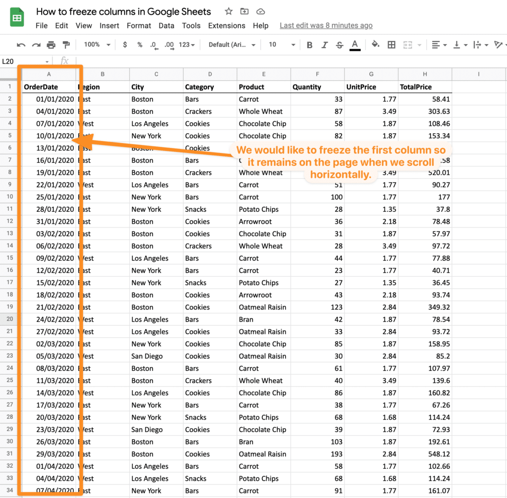
The most frequent use for freezing columns is to freeze the first column so any row titles that may be in the first column remain on screen when scrolling horizontally.
We will assume you have a Google Sheet ready and you would like to freeze one or more columns in the Google Sheet.
In our example we have a Google Sheet with some sales data and we wish to freeze the first column, which contains dates, so when we add more columns of data the first column remains static as we scroll horizontally.
There are two ways to achieve the same objective:
Method 1 – Using the mouse
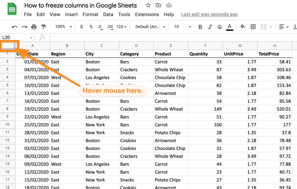
Hover over the top left square above the first row number.
Now move your mouse over the right border of this square.
When hovered over the right hand border click your left mouse button and drag the border across to the end of the first column border.
The first column in your Google Sheet is now frozen. If you scroll horizontally the first column remains on screen.
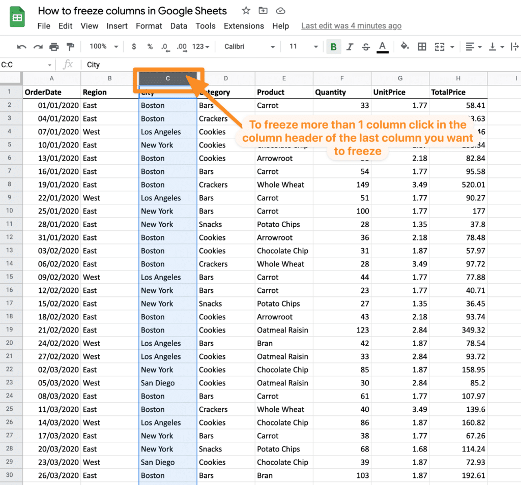
You can also use the mouse method to freeze more than one column in a Google Sheet. Simply drag the border of the top right box across to the end of the last column you want to freeze.
In our example below we are freezing the first three columns.
You will now see the first three columns of the Google Sheet are frozen.
Method 2 – Using the Google Sheets Menu
You can achieve exactly the same outcomes as we demonstrated above using the Google Sheets menu instead of the mouse method we explained above.
Open your Google Sheet and go to the “View” Menu and choose “Freeze” menu option.
You will see in the sub menu the option for “1 Column”.
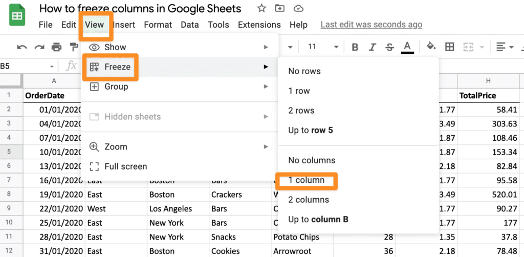
After selecting you will see the first column of your Google Sheet is now frozen.
If you want to freeze more than one column using the menu option (in our example below we will freeze the first three columns), first click in the column header of the final column you would like to freeze – e.g. to freeze columns A, B and C click in the column header of column C.
Now go to the “View” menu and then the “Freeze” sub menu and now choose “Up to Column C” – where column C will be the column where you clicked the header in the step above.
When selected you will see the first three columns of your worksheet are now frozen.
How to unfreeze columns in Google Sheets.
Unfreezing columns is really simple and is best achieved by using the menus in Google Sheets.
Go to the “View” menu and again chose the “Freeze” sub menu option. Now choose “No Columns”
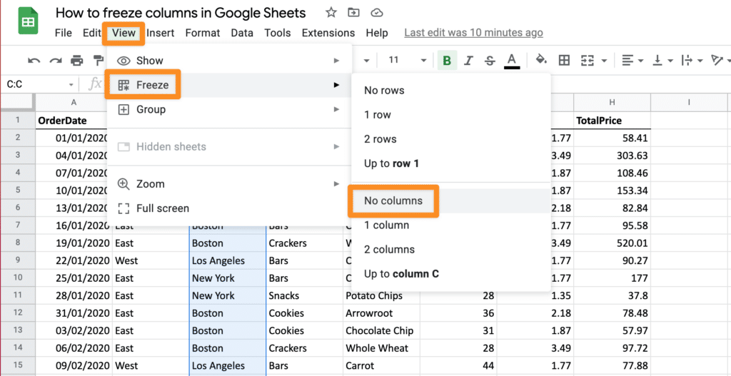
All the columns that were frozen will now be unfrozen.
More resources.
- The official Google documentation on freezing columns.
- Our YouTube video demonstrating the full process of freezing columns in Google Sheets.
We hope you found this DataSherpas quick tip useful. If you have any questions, please leave a comment below or contact us via our contact page.