How to freeze a row in Google Sheets
A DataSherpas Quick Tip.
In this quick tip article we will show you how to freeze a row in Google Sheets.
Sometimes for usability it helps to freeze one or multiple rows at the top of your Google Sheet. When you have a lot of rows of data, where the user of the Google Sheet needs to scroll, it helps to freeze rows so it is clear what column contains what data.
Before we start you should be aware there is a small limitation. You can freeze the top row of the sheet or any number of rows from the top, but, you cannot specifically freeze one row in the Google Sheet other than the top row. So for example you can freeze row 1 or rows 1-20 but not row 4 individually. Most people will not find this too limiting as the usual use case is to freeze the top row in the Google Sheet.
Let’s start with freezing the top row in your Google Sheet.
Here I have an example Google Sheet with food sales data. When I scroll down the sheet the top row scrolls off the screen too, so when I am viewing data further down the worksheet it is harder for me to understand what column contains what data.
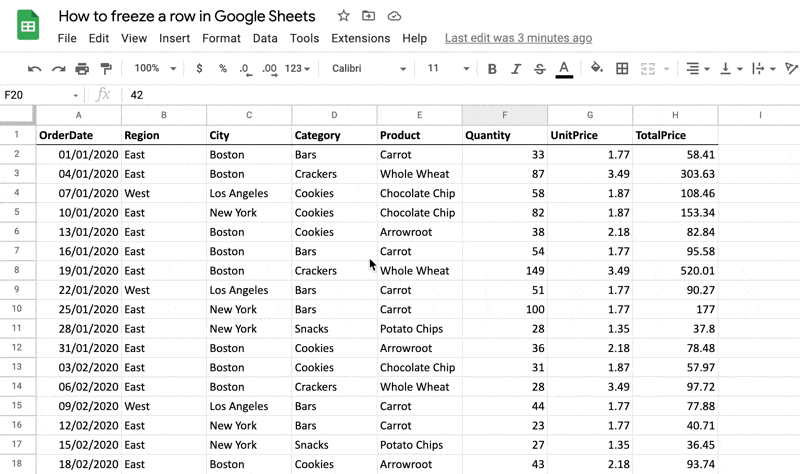
I want to freeze the top row of the worksheet so if I scroll further down the sheet the column headings remain visible.
As with most Google Sheets functionality there is more than one way to achieve the same result.
## Method 1 – use your mouse.
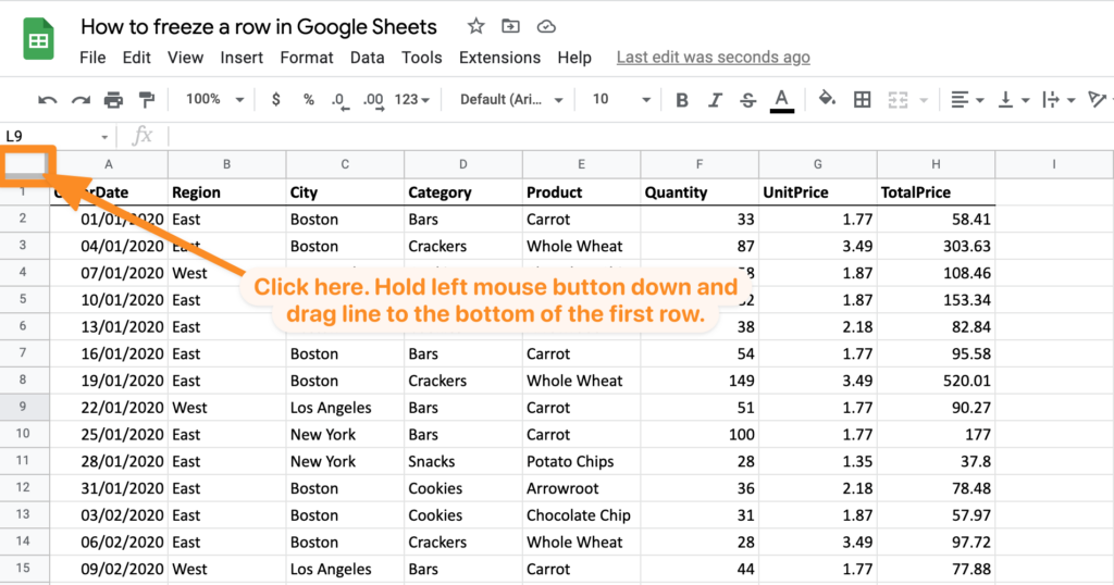
Google Sheets makes it really easy to freeze the top row with your mouse.
Just position your mouse in the left top corner of the worksheet, click your left mouse button and with the button still pressed drag downwards.
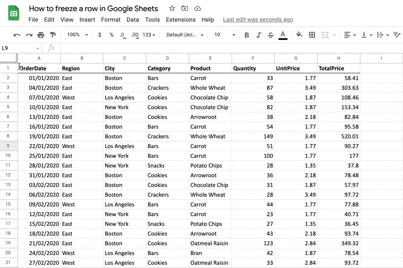
Now the top row becomes frozen and when I scroll down the Google Sheet the column headings remain visible.
Here is a quick animation of the process.
Method 2 – using the menu options.
You can achieve exactly the same outcome by using the menu options.
Go to the View menu, choose the “Freeze” menu option and then choose “1 Row”.
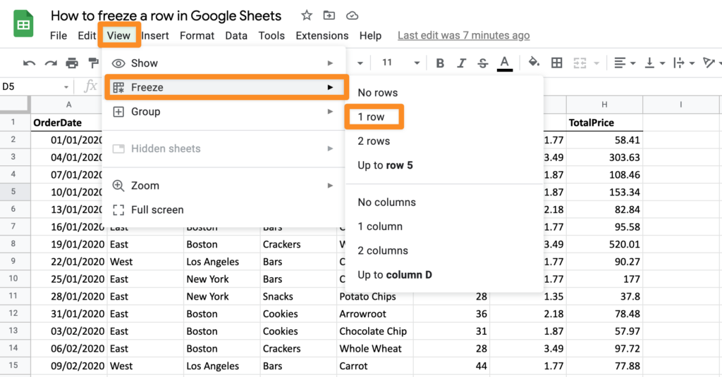
Now the first row will be frozen and column headers remain visible when scrolling further down the Google Sheet.
How to freeze more than one row.
You can also use the same methods to freeze more than one row at the top of your Google Sheet.
Let’s say I want to freeze the top three rows of the sheet.
Using the mouse just drag from the top left down to the third row.
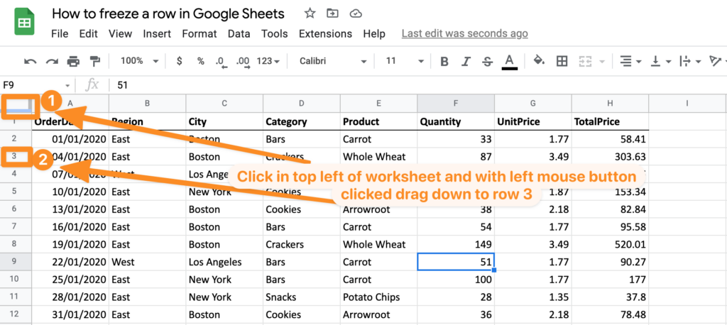
(In our example we are choosing to freeze the top 3 rows, but, you can freeze as many rows as you wish).
Here is an animation of the process.
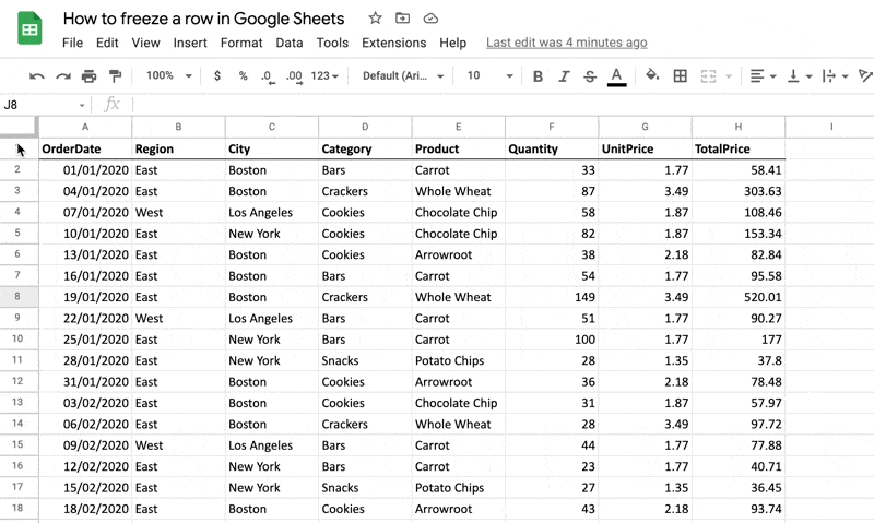
You can also do the same via the menu options.
Click anywhere in the row you want to freeze up to – e.g. if you want to freeze up to row 3, click somewhere in row 3.
Now to go to the View menu and choose “Freeze” and the choose “Up to row 3” (where the number 3 will reflect the row you clicked in above).
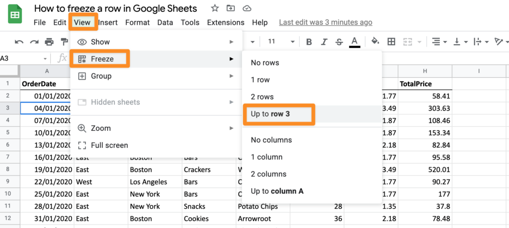
The top 3 rows will now be frozen and visible when you scroll further down the Google Sheet.
How to un-freeze rows in Google Sheets.
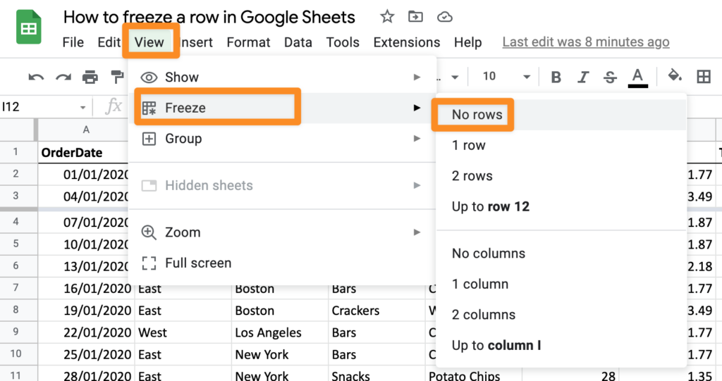
If you want to remove the rows you have chosen to freeze, simply go to the View menu at the top of your Google Sheet, then choose the “Freeze” menu option and then choose “No Rows”.
This will remove the “freeze” on all rows in the sheet.
More resources.
- The official Google documentation relating to freezing rows.
- Our Youtube video with a step by step walk through of the process.