A DataSherpas Quick Tip.
In this DataSherpas quick tip we take you through step by step instructions to show you how to create a drop down list in Google Sheets.
Drop down lists are a very popular for ensuring data input is consistent and validated in your Google Sheet and is particularly useful when you have many different people adding data to your Google Sheet.
Controlling data input is really important for reporting purposes – it is really hard to report on data entered as free form text. No matter how many instructions you add to your Google Sheet, over time you will see data anomalies like spaces, commas, etc. appearing in what is supposed to be structured data. Having drop down list options for data entry can help avoid this.
We will assume you already have a Google Account and know how to open a new Google Sheet.
There are two main steps to the process for creating a drop down list: 1) Create the options to appear in the list and 2) Add the drop down list to your sheet.
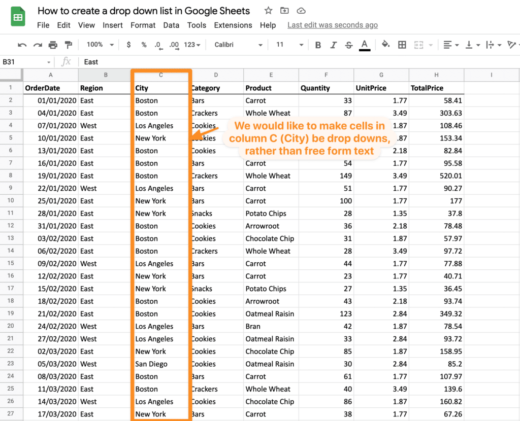
In our sample Google Sheet containing orders we would like to change the cells in column C, (City), to be a selected from a drop down instead of being a free form text entry.
First let’s create the options to appear in the drop down list.
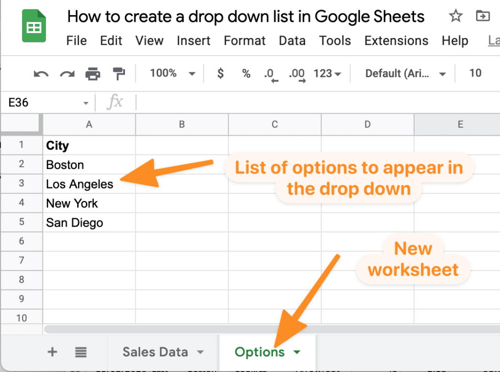
You can create the list of options on a new worksheet in the Google Workbook or you can add the options to your current worksheet. In our example we will choose to add to a new worksheet.
First we create the new worksheet and then in that new worksheet we add a column with the title and under the title the list of options we wish to be available as the drop down options on our main worksheet.
Now we are ready to add the drop down options to the relevant cells.
Next we flip back across to the main worksheet where we want to add the drop down list. This step is optional but we find it makes it easier and clearer to select the relevant options in the next step.
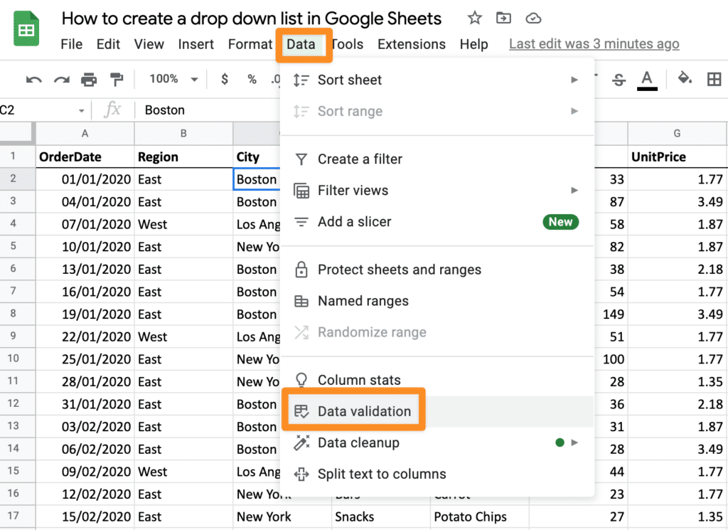
Next go to the “Data” menu at the top of your Google Sheet and choose the option “Data Validation”.
In the dialogue box that appears ensure you have the correct range of cells highlighted in the “Cell Range” option. These are the cells you want to turn into drop down lists.
You can change the selection by clicking in the box at the right of the “Cell Range” field – this allows you to select new cells if appropriate.
Always make sure your worksheet is referenced in the “Cell Range” , if you have more than one worksheet.
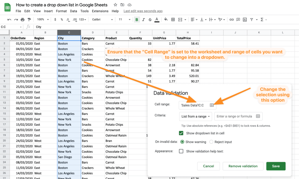
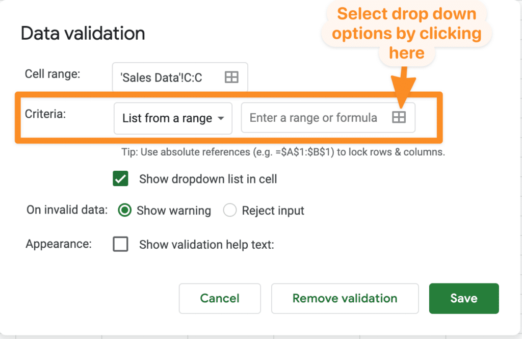
Next we need to choose the list of cells that contain the options to appear in the dropdown. Google calls this the “Criteria”.
Ensure you have “List from range” selected and then click on the box to the right of the text “Enter a range or formula”.
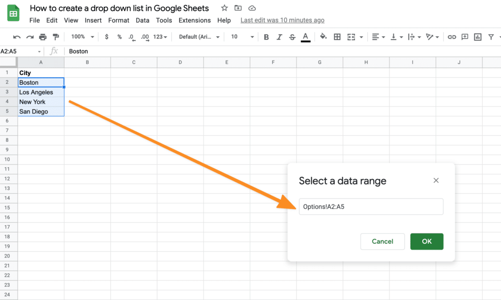
A new dialogue box appears asking you to select a range. Simply navigate to the worksheet (if appropriate) and column where you created your list of options (highlighted earlier in this process). Then select the cells in this list of options (except the title / column heading). Your selection will automatically be reflected in the “Select a data range” dialogue box.
When you have selected the correct cells click OK.
You will then be taken back to the main “Data Validation” dialogue box.
Ensure the “Show drop down list in cell” option is checked.
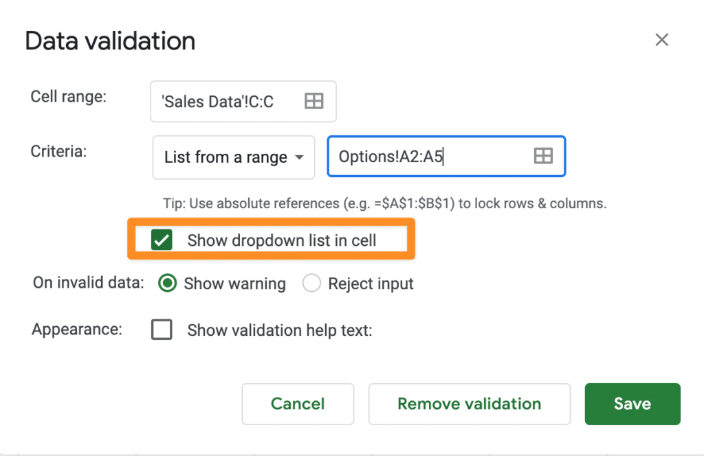
You can also choose to show a warning or reject input completely if data is entered that does not match the drop down options. In most cases you will want to choose “Reject input”, this will allow only selections from the drop down menu to be allowed as valid input.
You can also choose to show help text if appropriate.
When you are done with all of your selections, cross check carefully and then click “Save”.
Now the column you that you chose to have drop down cells should have all updated and drop down choices should be available in each cell in the column.
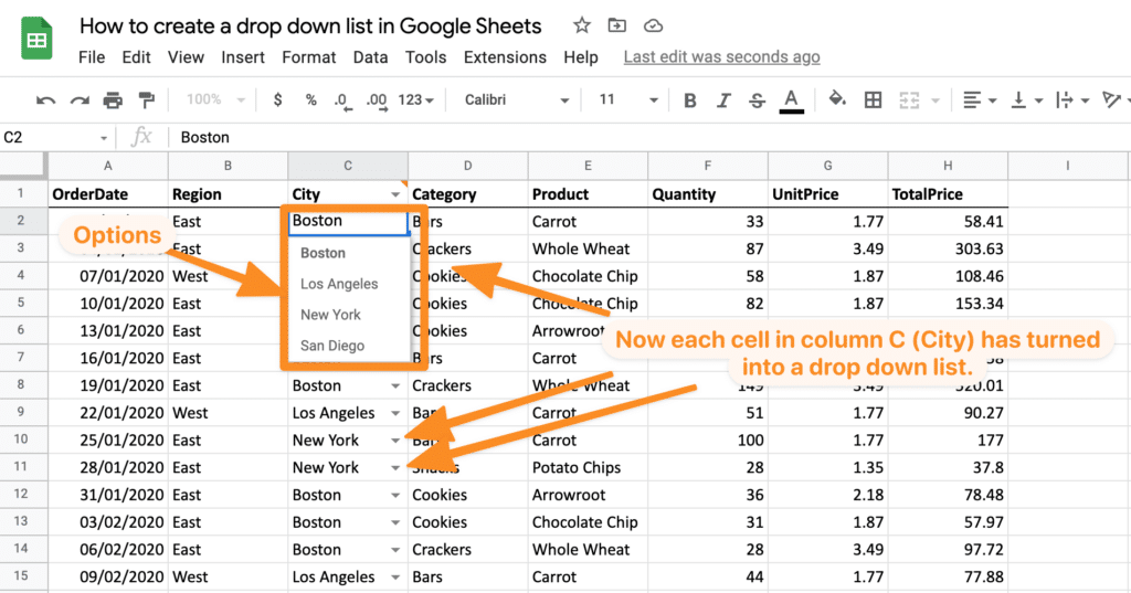
You will note, if you already had data in the range of cells, the data has been preserved.
Once you have completed this process once or twice it becomes very easy. In the example above we chose to make a whole column have drop downs. You can also choose just a few cells in a column, or row or just one cell. Data validation for creating drop downs can be applied to all type of cell scenarios and values of data.
Test different options dependent on your use case.
Other resources
- Our video on YouTube covering how to create a drop down list in Google Sheets.
- Google official support documentation on the topic.
We hope this DataSherpas quick tip has been useful. If you have any questions please leave us a comment below or send us a message via our contact page.