How to highlight every other row in Excel
A DataSherpas Quick Tip.
In this DataSherpas quick tip we show you how to highlight every other row in excel. Although row highlighting is mainly used for presentation purposes, highlighting alternate rows in an Excel worksheet can also help usability and help to highlight important data.
The process for highlighting every other row in Excel is very simple and will take just a few seconds. Let’s get started.
First open the Excel workbook and worksheet you want to apply the formatting to.
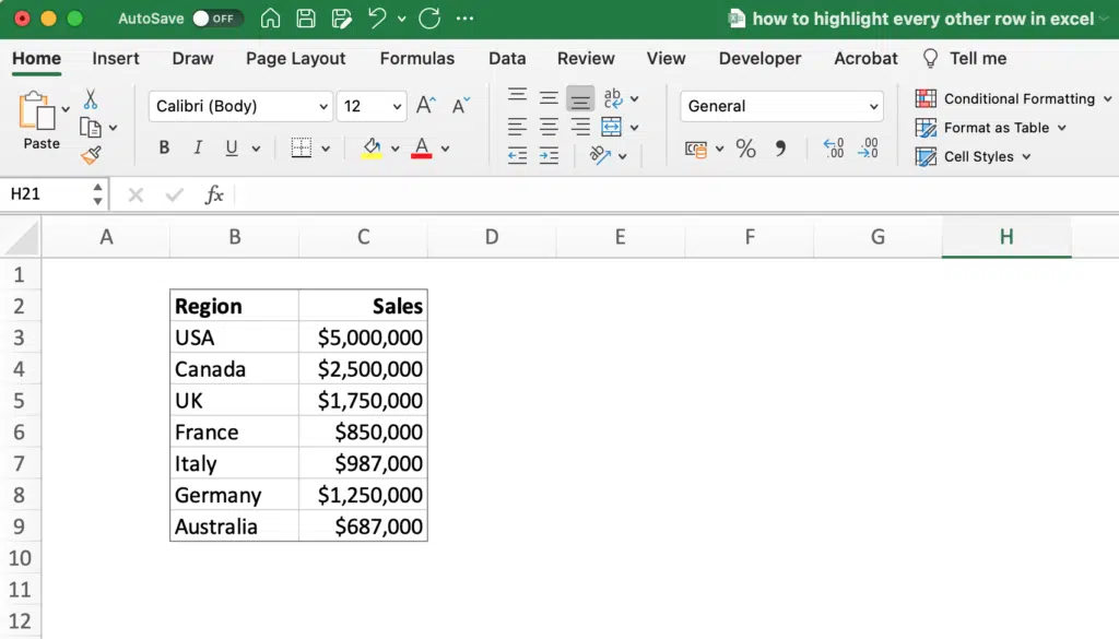
In our example below we have a simple set of data containing two columns where we would like to make every other row a different colour.
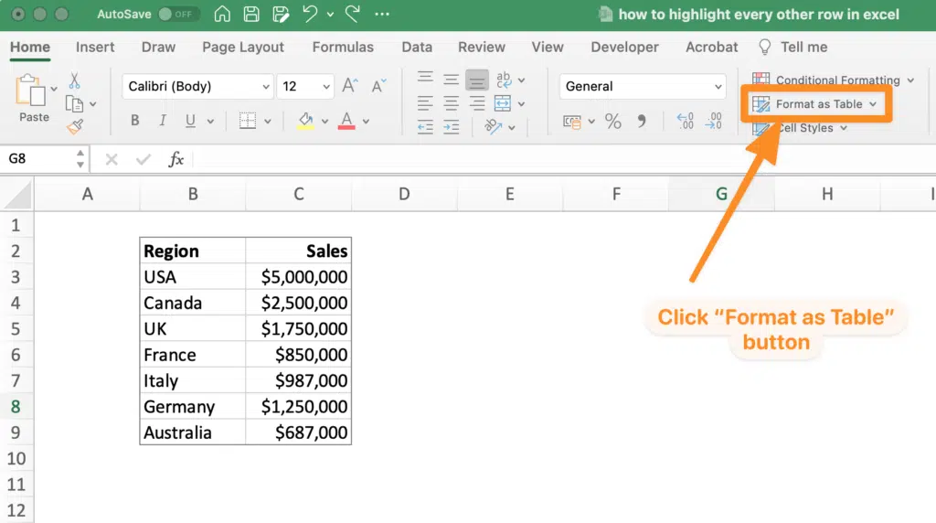
Step one in the process is to click on the “Format as Table” button on the ribbon bar at the top of your Excel worksheet.
When you click on the “Format as Table” button a new set of options appears with some pre defined formats you can quick apply to your selected data.
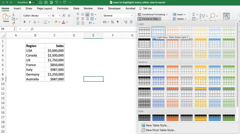
In ninety nine percent of circumstances one of these pre-built options will probably suit your requirements (we show you how to customize further a little later in this article).
Choose the styling, from the options provided, that is most appropriate for your needs. Note that some of the pre-defined styles do not highlight every other row by default.
In our example we will choose a style that highlights every other row in our data with a blue background.
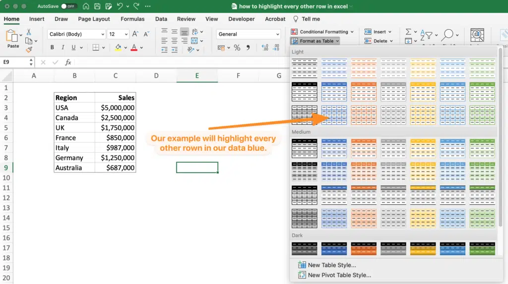
When you click on the style you wish to apply, a new dialogue box will appear asking you to choose the range of cells you wish to apply the styling to.
Simply click your mouse in the top left cell of the range of cells you want to apply the styling to and then, with your left mouse button held down, drag your mouse across and down to select all the cells to be formatted.
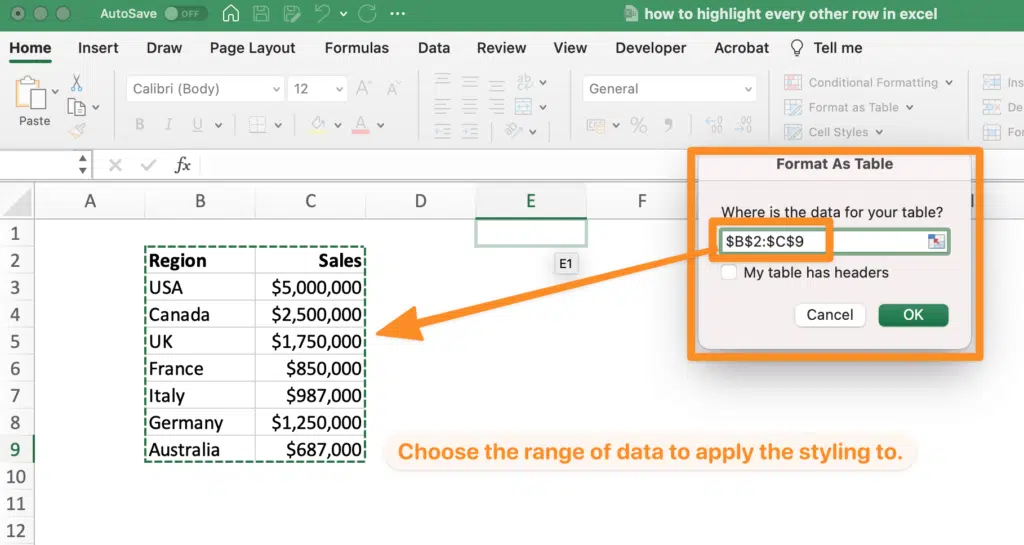
If your range of cells includes headers (or titles) for each column in your data, be sure to check the “My table has headers” checkbox too.
After you have selected the range of cells click OK on the dialogue box and the selected cells will have the chosen formatting applied.
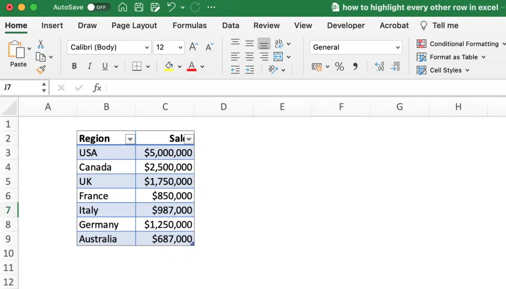
That is all it takes. You now have a nicely formatted table of data that makes analysing different rows easier.
Creating a custom style.
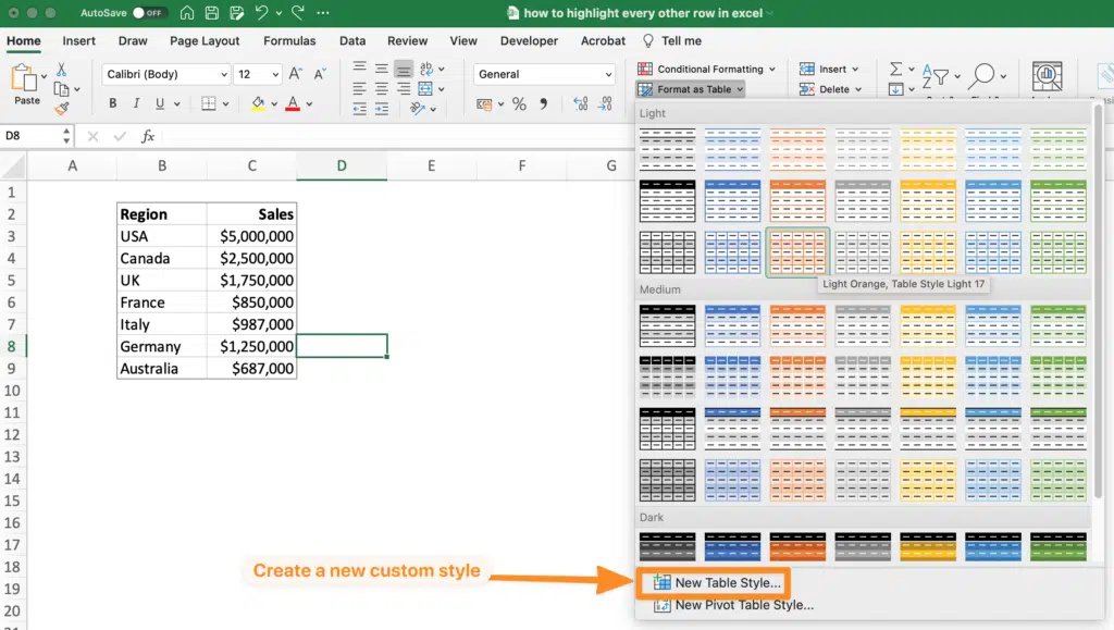
If none of the pre-built styles work for your specific needs then you can customise the styles and colors to suit your needs.
Simply click on the “Format as Table” button and then choose the “New Table Style” sub option.
This option then gives you the options to style specific parts of the table and apply custom formatting (font, borders, fills) the specific elements.
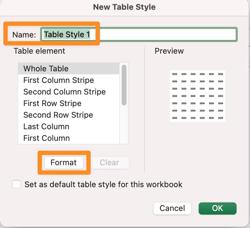
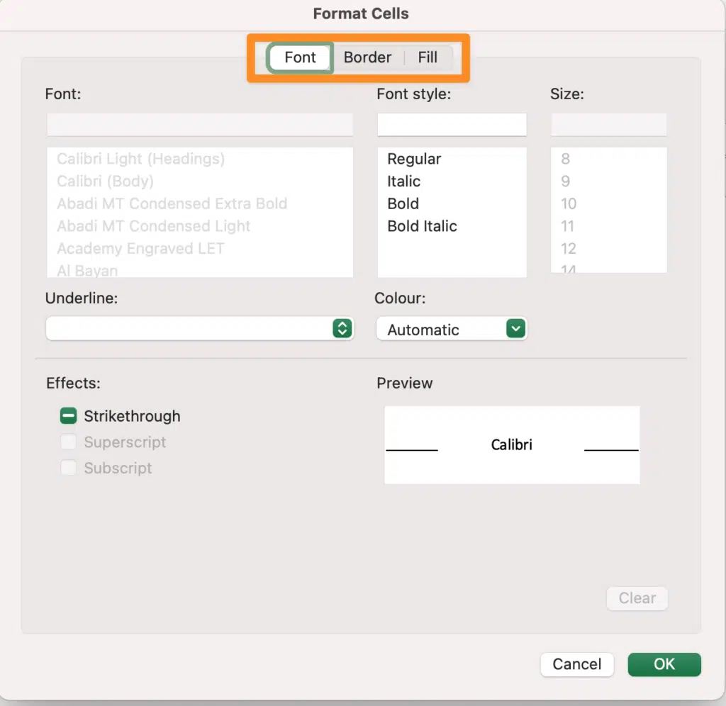
These options give you an almost infinite set of styling possibilities.
How to highlight every other row in the entire worksheet (not just a selection of cells)
If you want to highlight every other row in the entire Excel worksheet, and not just a small range of cells, you can easily do this but the method is slightly different. Instead of using table formatting we use conditional formatting.
First choose the worksheet you would like to apply the highlighting to and then click the square above the top left row number. This selects all cells in the worksheet.

Next go to the “Conditional Formatting” button on the ribbon at the top of your Excel worksheet and choose “New Rule” from the available sub options.

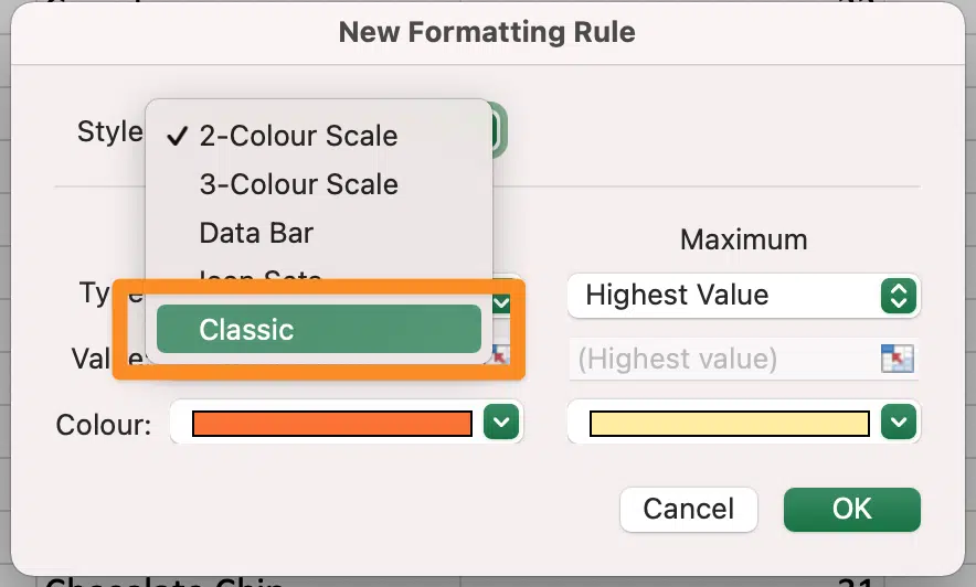
In the dialogue box that follows choose the “Classic” option for “Style”
Note: We are using Excel for Mac. Excel for Windows options may look slightly different but all options are available in both Excel for Mac and Windows.
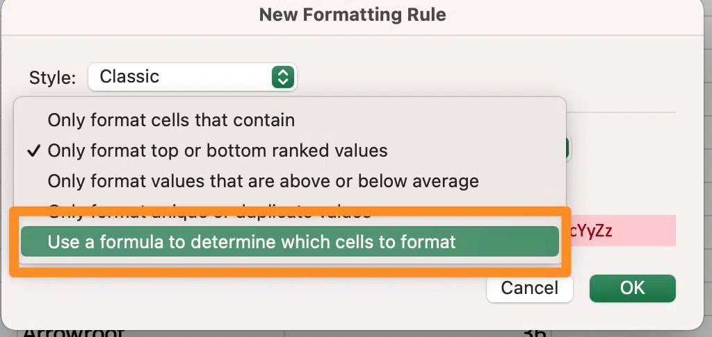
Then choose “Use a formula to determine which cells to format”
In the formula option enter the formula =MOD(ROW(),2)=0
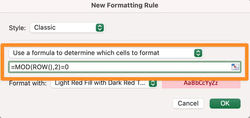
This formula determines if a row is odd or even (based on the row number) and then highlights the row accordingly.
Choose the colour scheme you wish to apply from the “Format with” box and then click “OK”
Every alternate row in your worksheet should now be highlighted.

We hope you found this DataSherpas quick tip useful. If you have any questions, or something is not working as expected, drop us a note in the comments or via our contact form and we will try our best to help.
Resources:
- The DataSherpas video with a step by step walk through of the process.
- The official Microsoft documentation for highlighting every other row.