How to wrap text in Google Sheets
A DataSherpas Quick Tip.
Quite often you will face the issue of how to display a long piece of text in Google Sheets. In this quick tip article we show you how to wrap text in Google Sheets. This allows you to display a large amount of text or other data, that will usually display across multiple columns, in one column with the text “folded” or “wrapped” so it is contained in one cell.
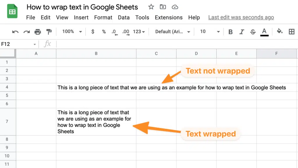
The process is very simple and will take less than 10 seconds.
We will assume you already have access to Google Sheets and have a sheet where you would like to apply text wrapping.
How to wrap text in a single cell.
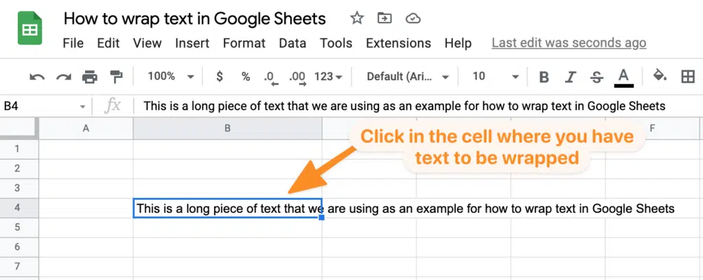
First open your Google Sheet and click in the cell where you would like to wrap the text.
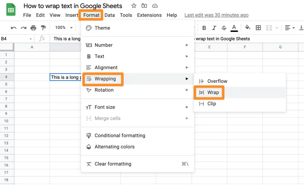
Next go to the “Format” menu at the top of the Google Sheet and choose the sub option “Wrapping” and then the “Wrap” option.
The text in the cell should now be wrapped.
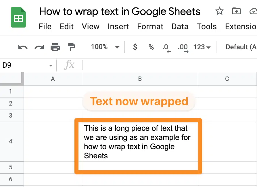
By wrapping the text in a single cell you also adjust the height of the rest of the cells in the same row. You can adjust this to suit your styling requirements by changing the column width for the column where the wrapped cell is present.
Wrapping text for all cells in a column or row.
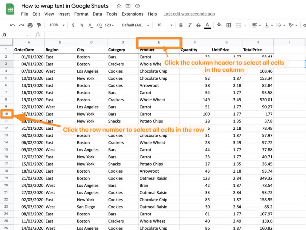
If you would like to wrap all of the text, in all cells in a specific column, or row in your Google Sheet (or even multiple columns or multiple rows) the process is exactly the same except you need to select all cells in the column / row and then go to the “Format > Wrapping > Wrap” menu option.
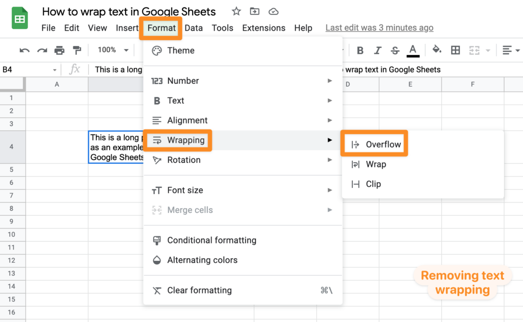
How to remove text wrapping
If you would like to remove the wrapping you have applied in your Google Sheet, select the cell or column or row with the wrapping applied. Now go to the “Format > Wrapping” menu and choose the “Overflow” option. This will remove the wrapping and change the text back to overflow multiple columns.
