How to total or sum a column in Google Sheets

A DataSherpas Quick Tip.

In this quick tip we show you how to total or sum a column in Google Sheets. Using a few simple shortcuts you can quickly and easily add together a set of numbers in a column to get a total. It takes just a few clicks of the mouse.

Let’s get started.

There are a few ways to be able to sum or total a column of numbers or values in Google Sheets. These are three of the most common and easiest methods.

Method 1 – Using the SUM function shortcut.

Using the sum function shortcut is arguably the easiest and quickest way to sum or total values in a Google Sheet column.

In our example we have a column called TotalPrice and we would like to sum or total the values in this column and display the total in cell H30.

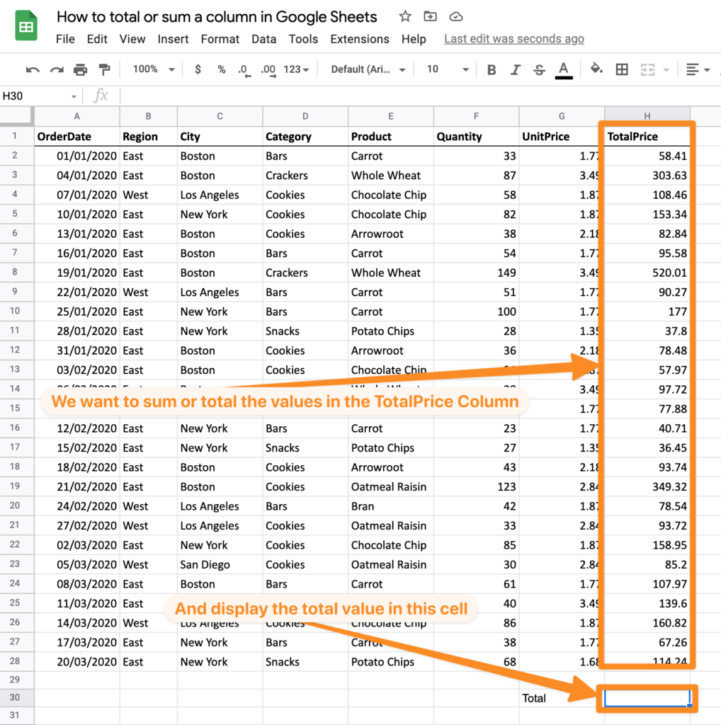
First of all I click in the cell where I would like the total displayed so in our case this is cell H30.

Next I go to the Google Sheets shortcut bar and click the functions shortcut button and then choose SUM from the sub menu.

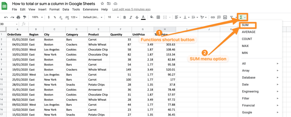
When you have chosen the SUM option Google Sheets will show a “helper” box in the cell where you want the total value displayed.

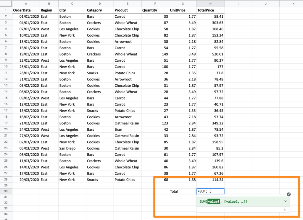
For now we can ignore this. The next step is to click on the top cell of the values in the column you want to sum and then drag your mouse down to the last value you want to sum.

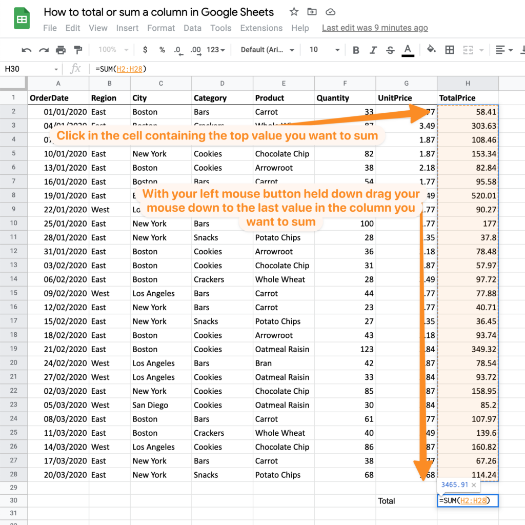
The cell where you want the total to appear should now reflect the range of cells you want to sum. In our example it is showing the range H2 to H28.

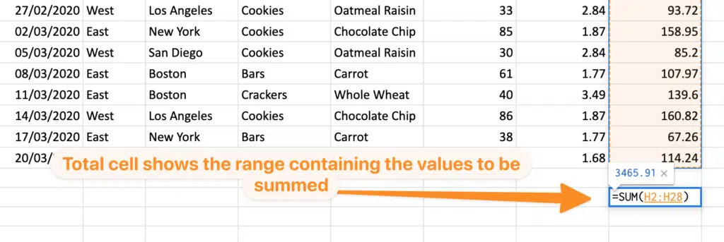
Now press enter on your keyboard.

The total of the values in the column should now show in your chosen cell.

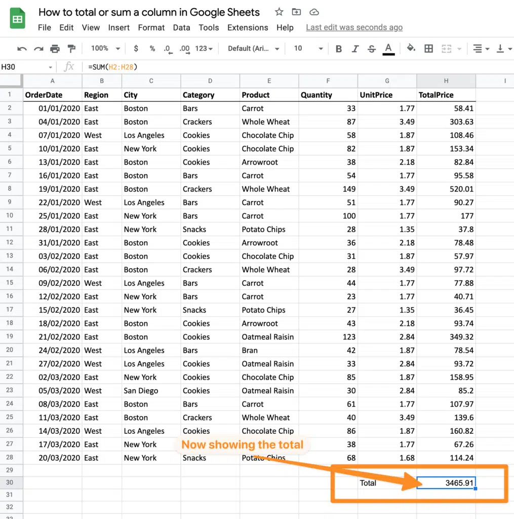
If you change any value in any of the cells in your column, the total value will automatically update.

Method 2 – Manually entering the range of cells to sum or total.

The second method involves manually entering the range of cells in the column you would like to sum or total.

First click in the cell where you would like the total to show.

In our example this is cell H30.

Next in that cell type the = sign. This tells Google Sheets that a function or calculation will follow in this cell.

Next we need to let Google Sheets know the type of function we will be using, in our case SUM.

Next we need to contain the cells to be summed in brackets so enter ( .

Next enter that cell reference for the top cell in the column. In our example this is H2.

Now we need to enter the : as a separator symbol followed by the cell reference for the last cell in the column to total. In our example this is cell H28.

Finally we need to close the brackets to let Google Sheets know this is the end of the function, so enter ) .

So the formula entered in our cell where the total is to appear is:

=SUM(H2:H28)

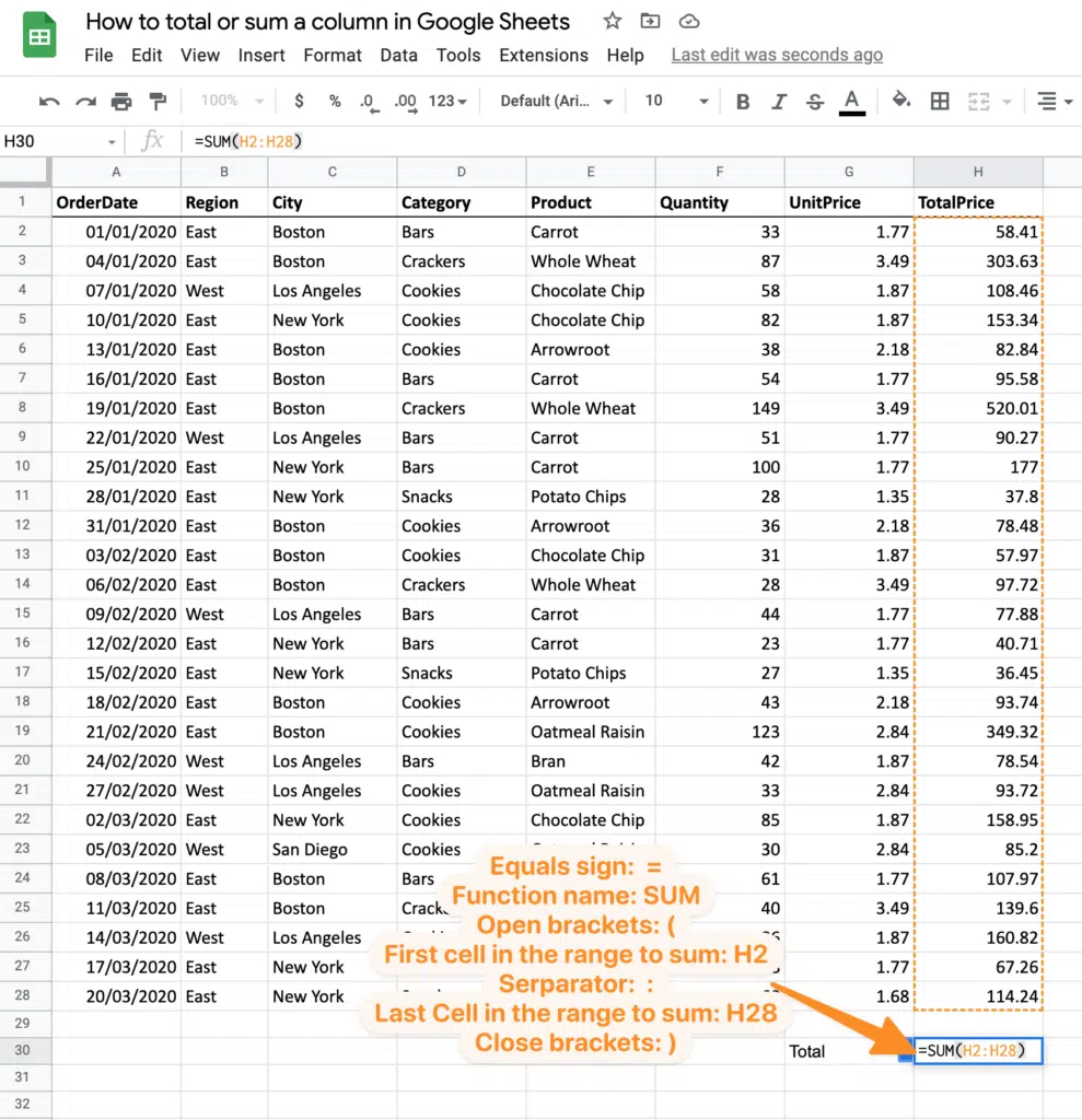
Now press enter and the total value will appear.

If you change any value in any of the cells in your column, the total value will automatically update.

Method 3 – Sum all values in a column.

In Method 2 we chose the start and end values in the column to sum or total. Now let’s suppose we just want to sum all values in the column, not a specific range. This is useful if you are adding new rows to your Google Sheet and you don’t want to manually update your formula in the total cell every time new rows are added.

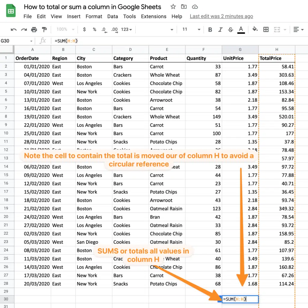
We follow the same steps as in method 2 above, but instead of our formula referencing specific cells in the column we just specify the whole column.

Note: do not to have your cell containing the total in the same column as the one you are trying to sum. You will get an error as Google Sheets will try to include the total cell in your calculation – so include itself in the total calculation. This creates a circular reference and will throw an error.

So your formula, using our example column, now becomes:

=SUM(H:H)

This tells Google Sheets to sum or total every value in column H.

Other resources:

Our YouTube video with a step by step walk through on how to total or sum a column in Google Sheets.
Official Google help pages on the SUM function.

———-

Related Quick Tips: